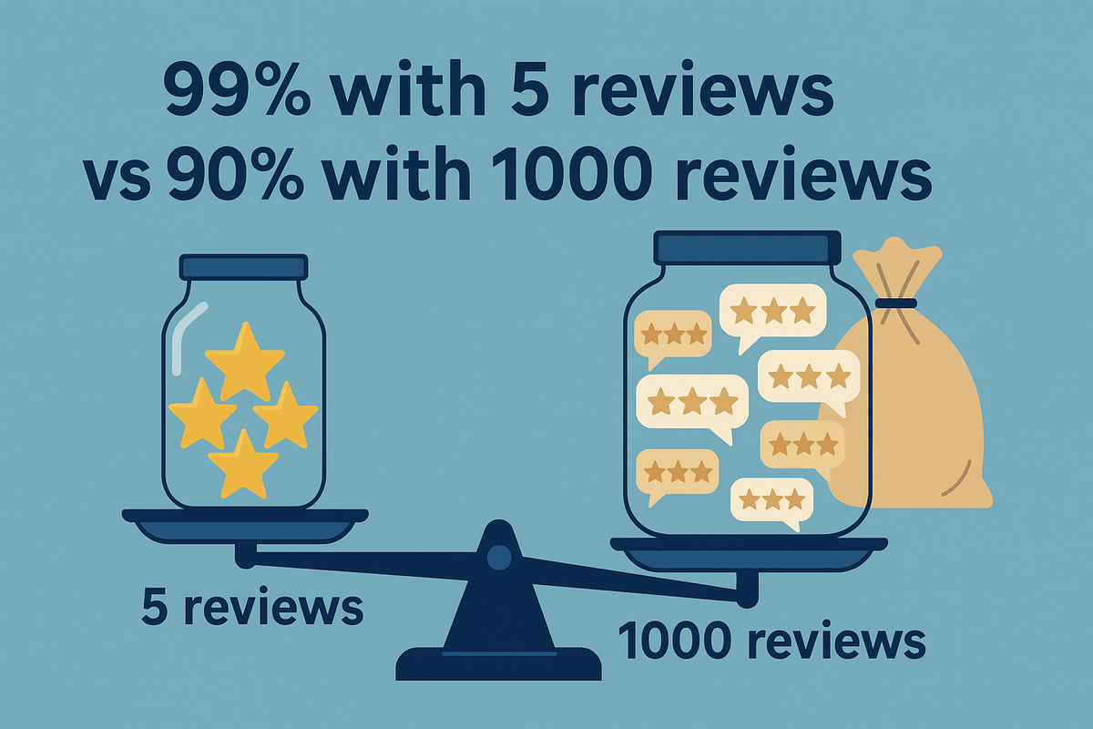
5 Reviews at 99% vs. 1000 Reviews at 90%: Which Seller is Better?

Motivation
Given the following reviews in Amazon, which seller is more likely to be a good seller?
| Seller | Number of Reviews | % of 5-star Reviews |
|---|---|---|
| A | 5 | 99% |
| B | 100 | 95% |
| C | 1000 | 90% |
This exploration was originally motivated by a practical question from my manager: how should we evaluate the risk profile of a borrower or seller? Specifically, if we have just a few records of a borrower defaulting, how confident can we be that this borrower represents a high risk?
To answer this question, we need to estimate the probability distribution of the probability (% of 5-star reviews or probability of default).
Intuition
The intuition here is that the more reviews a seller has, the more trustworthy their percentage of 5-star reviews becomes. Sometimes, 1000 reviews with 90% 5-star ratings is more reliable than 5 reviews with 99% 5-star ratings. From a Bayesian perspective, each review serves as a data point that updates our belief about the true probability of receiving a 5-star review.
Assuming a uniform prior, we can derive the posterior distribution of the probability of a 5-star review as follows:
Let \(p\) be the probability of a 5-star review, \(k\) be the number of 5-star reviews, and \(n\) be the total number of reviews.
- Uniform prior: \(P(p) = 1\)
- Likelihood: \(P(D|p) = p^k (1-p)^{n-k}\), where \(D\) represents the data. This is the binomial distribution.
- Posterior: \(P(p|D) = \frac{P(D|p)P(p)}{P(D)} = \frac{p^k (1-p)^{n-k}}{P(D)}\)
The term \(P(D)\) represents the marginal likelihood of the data, also known as the evidence. It acts as a normalization constant, ensuring that the posterior distribution integrates to 1. We calculate it by integrating the numerator over all possible values of \(p\):
\(P(D) = \int_0^1 P(D|p)P(p) ,dp = \int_0^1 p^k (1-p)^{n-k} \cdot 1 ,dp\)
The mean of the posterior distribution can be used to estimate the probability of a 5-star review given the available review data. We will derive this formula once we introduce the beta distribution. For now, note that \(E[p] = \frac{k+1}{n+2}\).
| Seller | Number of Reviews | % of 5-star Reviews | Number of 5-star Reviews | Mean Probability of Receiving a 5-star Review Next |
|---|---|---|---|---|
| A | 5 | 99% | 4.95 | 85% |
| B | 100 | 95% | 95 | 94% |
| C | 1000 | 90% | 900 | 90% |
Based on this analysis, seller B would be the optimal choice.
Beta Distribution
The Probability Density Function (PDF) of the beta distribution is given by:
$$f(p;\alpha,\beta) = \frac{1}{B(\alpha,\beta)} p^{\alpha-1} (1-p)^{\beta-1}$$
where \(B(\alpha,\beta)\) is the beta function, and \(\alpha\) and \(\beta\) are the shape parameters.
The beta function is defined as:
$$B(\alpha,\beta) = \int_0^1 p^{\alpha-1} (1-p)^{\beta-1} dp$$
The PDF gives the probability of a probability \(p\) occurring given the shape parameters \(\alpha\) and \(\beta\). The beta function is a normalization constant that ensures the PDF integrates to 1.
The Core Shape: \(p^{\alpha-1} (1-p)^{\beta-1}\)
- \(p\) is the probability we are estimating (e.g., probability of a 5-star review).
- \(\alpha-1\) relates to the count of successes (e.g., number of 5-star reviews).
- \(\beta-1\) relates to the count of failures (e.g., number of non-5-star reviews).
If \(\alpha\) is large and \(\beta\) is small, the term \(p^{\alpha-1}\) dominates when \(p\) is close to 1, pushing the peak of the distribution towards 1. Conversely, if \(\alpha\) is small and \(\beta\) is large, the term \(p^{\alpha-1}\) dominates when \(p\) is close to 0, pushing the peak of the distribution towards 0. If \(\alpha=1\) and \(\beta=1\), the distribution is uniform, 1.
Why the Beta Distribution is Defined As It Is
1. The Starting Point: The Data Generation Process
The story begins not with the Beta Distribution, but with the process it aims to model: sequences of successes and failures. This is the Binomial Process.
If you know the underlying probability of success, \(p\), the likelihood of observing \(k\) successes in \(N\) trials is given by the Binomial Distribution:
$$P(k \text{ successes in } N \text{ trials}) = \binom{N}{k} p^k (1-p)^{N-k}$$
Since \(\binom{N}{k}\) is a constant, we can rewrite the likelihood as:
$$\text{Likelihood}(p) \propto p^k (1-p)^{N-k}$$
2. The Inverse Problem (Thomas Bayes and Pierre-Simon Laplace)
If we observe the data (\(k\) successes in \(N\) trials), what can we say about the unknown probability of success, \(p\)?
This requires using what we now call Bayes' Theorem:
$$\text{Posterior}(p) \propto \text{Likelihood}(p) \times \text{Prior}(p)$$
To solve this, we need a starting assumption about \(p\) before seeing any data (the prior). If we know absolutely nothing about \(p\), we can use a uniform prior, which is a constant.
$$P(p|D) \propto p^k (1-p)^{N-k}$$
3. The Desire for Mathematical Elegance: Conjugacy
While the distribution emerged naturally from the Binomial process, mathematicians also approached this from the perspective of desired properties. When modeling a probability \(p\), we want a distribution that is easy to update. We want a form for the prior such that when multiplied by the likelihood, the resulting posterior has the same mathematical form as the prior.
Given the likelihood \(p^k (1-p)^{N-k}\), the structure that is conjugate to it is the Beta distribution.
4. The Kernel
Mathematicians abstracted the exponents into two shape parameters, \(\alpha\) and \(\beta\):
$$\text{Kernel}: p^{\alpha-1} (1-p)^{\beta-1}$$
Why the "-1"? This is a mathematical convention that makes the parameters \(\alpha\) and \(\beta\) behave elegantly. For example, the uniform distribution becomes \(\text{Beta}(1,1)\). Additionally, if \(\alpha = 0\) and \(\beta = 0\), the distribution becomes undefined, since:
$$B(0,0) = \int_0^1 p^{-1} (1-p)^{-1} dp = \int_0^1 \frac{1}{p(1-p)} dp$$
This integral diverges, which is why we need \(\alpha, \beta > 0\).
5. Normalization
We have the shape (the kernel), but this alone is not a Probability Density Function (PDF). A PDF must integrate to exactly 1 (the total area under the curve must be 100%).
To turn this kernel into a proper PDF, we need a normalization constant. This requires calculating the integral of the kernel from 0 to 1:
$$\int_0^1 p^{\alpha-1} (1-p)^{\beta-1} dp$$
This integral evaluates to the Beta function, \(B(\alpha, \beta)\):
$$B(\alpha, \beta) = \int_0^1 p^{\alpha-1} (1-p)^{\beta-1} dp$$
Therefore, the complete Beta Distribution PDF is:
$$f(p|\alpha, \beta) = \frac{1}{B(\alpha, \beta)} p^{\alpha-1} (1-p)^{\beta-1}$$
The normalization constant \(\frac{1}{B(\alpha, \beta)}\) ensures that the total area under the curve equals 1, making it a valid probability distribution.
Mean and Variance
The mean of the beta distribution is given by:
$$E[p] = \frac{\alpha}{\alpha+\beta}$$
The mean of a PDF is given by:
$$\begin{align}E[p] &= \int_0^1 p \cdot f(p|\alpha, \beta) , dp\\&= \int_0^1 p \cdot \frac{1}{B(\alpha, \beta)} p^{\alpha-1} (1-p)^{\beta-1} , dp\\&= \frac{1}{B(\alpha, \beta)} \int_0^1 p^{\alpha} (1-p)^{\beta-1} , dp\\&= \frac{B(\alpha+1, \beta)}{B(\alpha, \beta)} \quad \text{(using the beta function identity)}\\&= \frac{\alpha}{\alpha+\beta} \quad \text{(using the beta-gamma identity: } B(\alpha, \beta) = \frac{\Gamma(\alpha)\Gamma(\beta)}{\Gamma(\alpha+\beta)}\text{)}\end{align}$$
Earlier, we discussed that the mean probability of a 5-star review given \(k\) five-star reviews out of \(n\) total reviews is \(\frac{k+1}{n+2}\). This is precisely the mean of a Beta distribution with parameters \(\alpha = k+1\) (successes + 1) and \(\beta = (n-k)+1\) (failures + 1). This elegant connection is known as Laplace's Rule of Succession.
The variance of the beta distribution is given by:
$$Var[p] = \frac{\alpha\beta}{(\alpha+\beta)^2(\alpha+\beta+1)}$$
To derive the variance, we leverage the fact that the variance of a PDF is given by:
$$Var[p] = E[p^2] - E[p]^2$$
We can derive \(E[p^2]\) using the same approach as \(E[p]\):
References
From Easy to Hard and Theoretical to Practical:
- Beta Distribution: an Intuitive Explanation
- The Beta Distribution: Lecture Notes #21
- Laplace's Rule of Succession
- Limitations of Laplace's Rule of Succession
- Reading 15: Conjugate priors: Beta and normal
- The Joys of Conjugate Priors
- How long does it take to become Gaussian?
- A Bayesian view of Amazon Resellers
- Find a beta distribution that fits your desired confidence interval
- Practical Use of the Beta Distribution for Data Analysis