Another Suspicious Correlation in Risk: An Example to Illustrate the Causal Graph and Path-Tracing Rule

In the offline cellphone-loan business, we have observed that default risk increases with the premium features of the device used during loan application. For example, borrowers applying with phones that have larger storage capacities tend to show higher default rates—counter to the intuitive expectation that “better” devices signal lower risk.

At first glance, this pattern might be dismissed as selection bias: the set of people who apply for a loan with a premium device is not the same as the set of people who own a premium device but never seek financing.

I initially sketched the following causal graph:

graph LR
    A["Premium Device"] --> |neg| B["Loan"]
    B --> |pos| C["Risk"]

Yet this diagram is unsatisfactory, because conditioning on the Loan node blocks any causal path from Premium Device to Risk. (For reader unfamiliar with causal graphs, please refer to Appendix for more details.)

The next day, it struck me that “risk” has two distinct meanings:

• (Risk_t) – the borrower’s inherent (pre-loan) risk
• (Risk_{t+1}) – the observed risk after the loan is taken

Rewriting the graph:

  graph LR
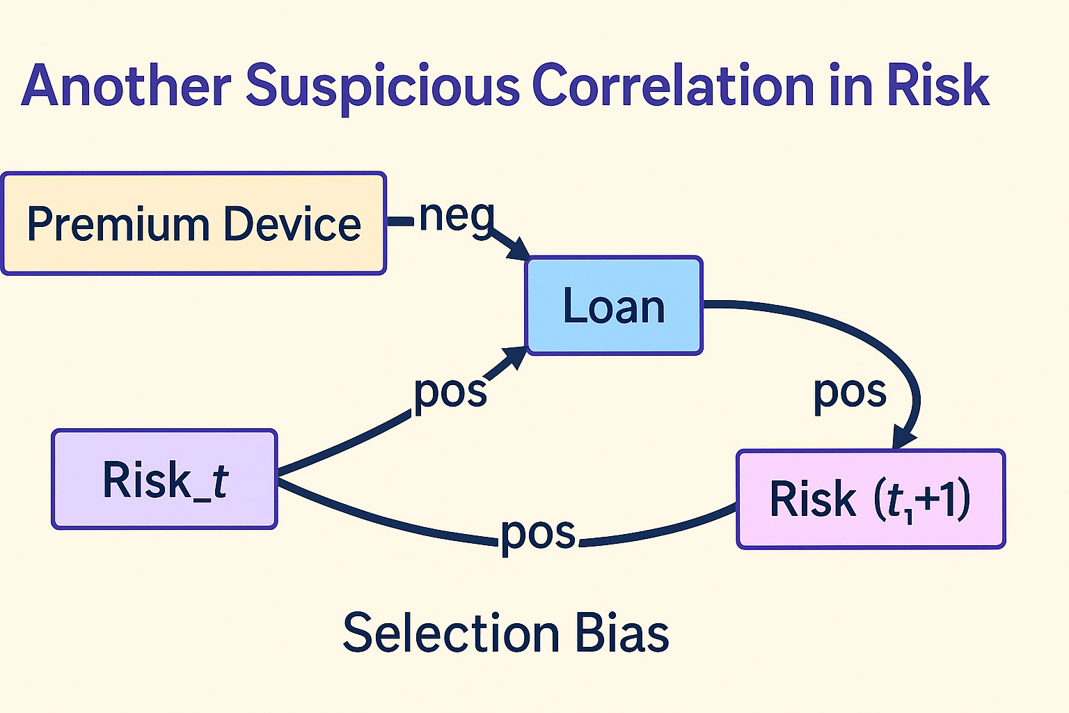
      A["Premium Device"] --> |neg| B["Loan"]
      B --> |pos| C["Risk_{t+1}"]
      D["Risk_t"] --> |pos| B
      D --> |pos| C

Conditioning on the population that takes a loan opens a back-door path from Premium Device to (Risk_{t+1}), producing the positive correlation (See Appendix for explanation). However, the assumption can not be validated because the population that does not take a loan is not observable and the same explanation can be applied to any suspicious correlation.

More broadly, many puzzling risk correlations can be traced to this same collider structure. A hidden variable—call it Ability / Income—influences both a customer’s device choice and their baseline risk. Once we condition on “takes a loan,” that collider again induces a spurious link:

  graph LR
  subgraph "Latent Variables"
    X(("Ability / Income"))
  end
  X --> |pos| Device["Premium Device"]
  X --> |neg| Risk_t["Risk_t"]
  Device --> |neg| Loan["Loan"]
  Risk_t --> |neg| Loan
  Loan --> |pos| Risk_t1["Risk_{t+1}"]
  Risk_t --> |pos| Risk_t1
  X --> |neg| Loan

Understanding the data generating process is key to identifying the causal graph. I would argue that understanding the data generating process, which is equivalent to understanding the mechanisms and causal relationships between variables, is the most important skill for making impactful contributions across many fields.

Appendix

Causal Graphs

A causal graph is a directed acyclic graph (DAG) that represents the causal relationships between variables. Each node represents a variable, and each arrow represents a causal relationship.

Common Causal-Path Patterns in Causal Graphs

Essentials to remember

• Adjust for confounders (forks) but not for colliders (v-structures).
• Mediators transmit effect; controlling for them blocks part of the causal influence.
• Back-door criteria: block every non-causal path that ends with an arrow into X.
• Front-door criteria: use a mediator that fully transmits X’s effect and is untouched by hidden confounders.
• Selection on any descendant of a collider likewise induces spurious associations (selection bias).

These patterns cover nearly all day-to-day causal puzzles: identify which structure you have, then decide whether to adjust, stratify, or leave the variable untouched.

Identifying the relationship between variables: Wright’s Path-Tracing Rule

Sewall Wright (1921 – 1934) developed path analysis to decompose correlations in a (linear) causal diagram into products of edge coefficients.
The path-tracing rule tells you exactly which paths count and how to sum them to get a covariance (or correlation) between any two variables.

Set-up & Assumptions

Linear structural equations
Each node is a standardized variable (mean 0, var 1) with an equation
\(X_i = \sum_{j\in\mathrm{pa}(i)} \beta_{ji}X_j + \varepsilon_i\),
where the \(\beta\)'s are path coefficients.

1. No feedback (the graph is acyclic)
   One-headed arrows show direct causal effects.
2. Error terms \(\varepsilon_i\) are mutually independent
   And uncorrelated with causes.

Under these conditions, every observed correlation is the sum of products of edge coefficients along all "admissible" open paths between the variables.

Admissible Paths

A path from X to Y is admissible if it satisfies all of Wright's rules:

If you are working in an ordinary DAG with independent errors, Rule 3 and Rule 4 never arise, so an admissible path is simply a chain of single-headed arrows with no repeats.

The Algebra

For two standardized variables A and B:

$$\operatorname{cor}(A,B) = \sum_{\text{admissible paths }p} \prod_{e\in p}\beta_e$$

Where:

• Product: Multiply the signed coefficients along each admissible path.
• Sum: Add those products across all paths.

Because the variables are standardized, covariances equal correlations.

Tiny Worked Example

  graph LR
    X -->|0.4| M
    M -->|0.5| Y
    X -->|0.3| Y

Admissible X → Y paths:

1. Direct: \(X \xrightarrow{0.3} Y\) → contribution 0.3
2. Indirect: \(X \xrightarrow{0.4} M \xrightarrow{0.5} Y\) → contribution 0.4 × 0.5 = 0.20

$$\operatorname{cor}(X,Y) = 0.3 + 0.20 = 0.50$$

Sign of the conditional covariance

For a single conditioning variable \(Z\) in the linear/Gaussian setting,

$$\operatorname{Cov}(X,Y\mid Z)=\operatorname{Cov}(X,Y)-\frac{\operatorname{Cov}(X,Z),\operatorname{Cov}(Y,Z)}{\operatorname{Var}(Z)}.\tag{★}$$

Because the second term is subtracted, its sign is the opposite of
\(\operatorname{Cov}(X,Z)\times\operatorname{Cov}(Y,Z)\).

If the unconditional covariance is already non-zero, the flip still follows the table once you compare its size to the adjustment term.

How this ties to colliders

A collider is a node that both (X) and (Y) point into:

  graph TD
    X --> Z
    Y --> Z

1. Marginally (ignoring \(Z\)) the arrows end at \(Z\), so \(X\) and \(Y\) are d-separated → uncorrelated.
2. Conditioning on \(Z\) "opens" the path \(X \rightarrow Z \leftarrow Y\), creating a correlation whose sign is exactly what (★) predicts:

$$\operatorname{Cov}(X,Y\mid Z)\approx-\frac{\operatorname{Cov}(X,Z),\operatorname{Cov}(Y,Z)}{\operatorname{Var}(Z)}.$$

Intuition: inside any stratum of \(Z\), if \(X\) takes a value that raises \(Z\), \(Y\) must take a value that lowers \(Z\) to keep \(Z\) fixed, so they look like substitutes (negative correlation) when their pushes go the same way, and like complements (positive correlation) when they push in opposite ways.

Concrete numeric example

Suppose in the population

• \(X,Z,Y\sim\mathcal{N}(0,1)\)
• \(\operatorname{Cov}(X,Z)=\operatorname{Cov}(Y,Z)=0.5\)
• \(\operatorname{Cov}(X,Y)=0\)

Then

$$\operatorname{Cov}(X,Y\mid Z)=0-\frac{0.5\times 0.5}{1}=-0.25$$

Adjusting for the collider \(Z\) turns two independent variables into negatively correlated ones.

Flip one sign, e.g. \(\operatorname{Cov}(Y,Z)=-0.5\), and the conditional covariance becomes \(+0.25\).