Lease Decay

In Singapore's property market, properties are classified into two categories: leasehold and freehold. Freehold grants perpetual ownership of both the property and land. In contrast, leasehold means the owner owns the property but leases the land from the government, typically for 99 years. Once the lease expires, the land reverts to the government. Because leasehold owners do not have perpetual ownership, they usually anticipate a discount in property value compared to freehold properties. How can we quantify this discount?
Discounted Cash Flow
For perpetual ownership, the present value (PV) of the property is calculated as \[PV = \sum_{t=1}^{\infty} \frac{C_1(1+g)^{t-1}}{(1+r)^t} = \frac{C_1}{r - g}\], where \(g\) represents the growth rate of the annual cash flow starting with \(C_1\), and \(r\) is the discount rate (All rates are real). You can derive it using the closed-form solution of the geometric series.
For leasehold, the PV of the property with maturity (remaining lease year) \(T\) is calculated as \[PV(T) \;=\; \sum_{t=1}^{T} \frac{C_1 (1+g)^{t-1}}{(1+r)^t}\;=\; \frac{C_1}{r-g}\left[\,1 - \left(\frac{1+g}{1+r}\right)^{T}\,\right]\]
Dividing leasehold with freehold, we get the ratio:
\[\frac{\text{Leasehold}(T)}{\text{Freehold}}= 1 - \left( \frac{1+g}{1+r} \right)^{T}\]
Using continuous compounding is more convenient because it allows us to express the return as \(r - g\). The formula is:
\[\frac{P^{\mathrm{Lease}}(T)}{P^{\mathrm{Free}}}= 1 - e^{-(r - g)T}\]
Estimating \(r-g\)
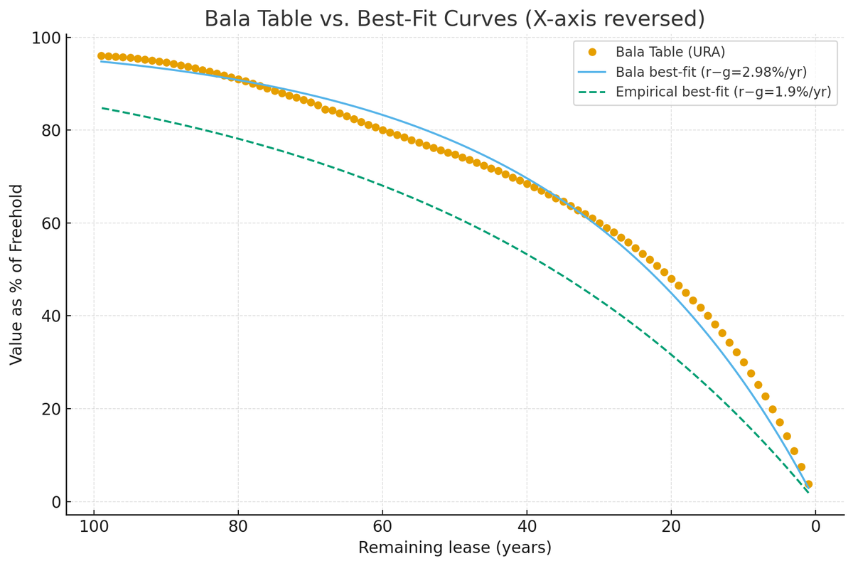
The Urban Redevelopment Authority (URA) publishes a Bala table, LEASEHOLD VALUES AS PERCENTAGE OF FREEHOLD VALUE. Best-fit constant net rate \(r-g \) from Bala Table is approximately 2.98%/yr (continuous compounding), fitted by least squares to all terms \(T = 1…99\)
Empirical study on lease decay ( Stefano Giglio & Matteo Maggiori & Johannes Stroebel, 2015. "Very Long-Run Discount Rates," The Quarterly Journal of Economics, Oxford University Press, vol. 130(1), pages 1-53.) shows that to match the long-maturity discounts, you need a constant \(r−g≈1.9\%\) per year.
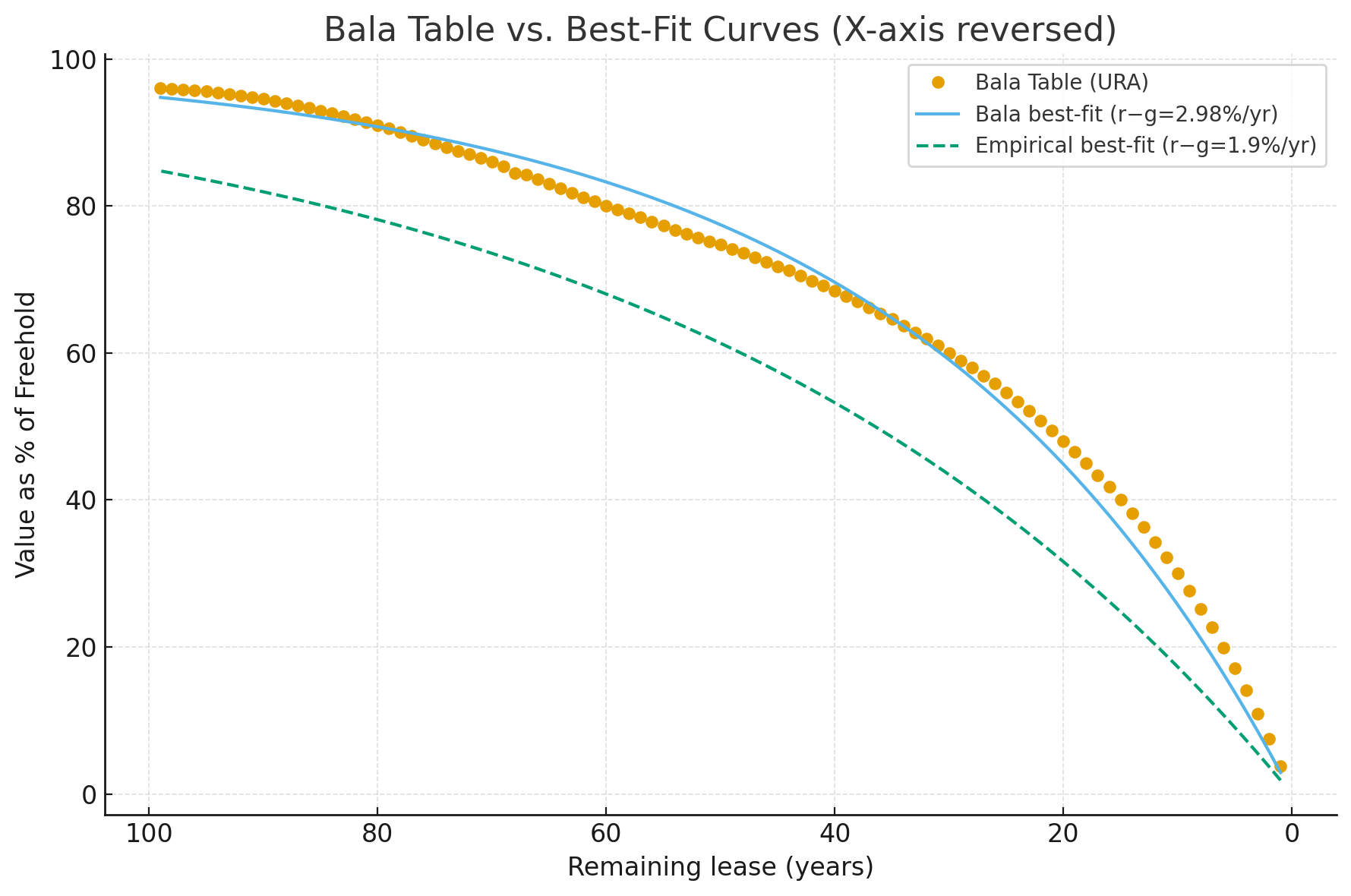
We can decompose the freehold value into the leasehold value and the value of holding the property perpetually after the lease expires. A higher discount rate reduces the present value of future cash flows, making people prefer immediate cash flow more. As a result, as time passes (the remaining T shrinks), the value decreases.
Processing housing loans within the Total Debt Servicing Ratio framework employs a 3.5% "stress test" interest rate (nominal). The actual interest rate in 2025 is around 2% (nominal). Over the past 10, 20, and 30 years, the average inflation rates have been 1.58%, 2.12%, and 1.71%, respectively. For the inflation-adjusted rental growth rate, the empirical data show 0.2% per year.
Using these data points, we can perform a Monte Carlo simulation grounded on our prior for the distribution of the d-g. I prefer the Beta distribution. You can find the reasoning and calculator here. Assuming no rental growth, the value at the lower end of my confidence interval is 1.5%. The value at the higher end of my confidence interval is 2.5%. The beta distribution is \(beta(41.087497781332885, 2040.563860086082)\)
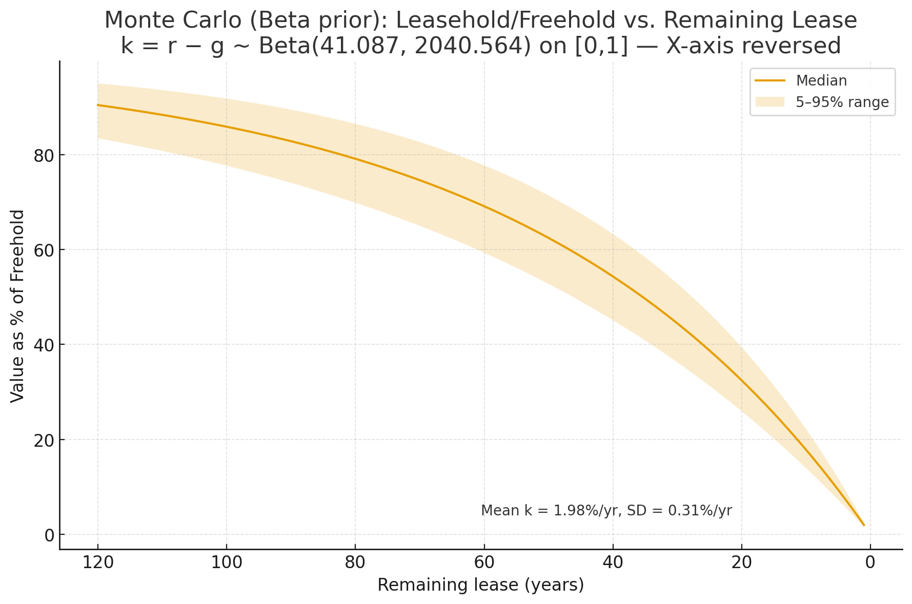
Simulated with k = r - g using a Beta distribution: Beta(41.0875, 2040.5639) on [0,1]. The mean value of k is approximately 1.98% per year, with a standard deviation around 0.31% per year.
|
Term of Years |
Percentage (%) of Freehold Value |
Term of Years |
Percentage (%) of Freehold Value |
Term of Years |
Percentage (%) of Freehold Value |
|
1 |
2.0 |
34 |
49.0 |
67 |
73.5 |
|
2 |
3.9 |
35 |
50.0 |
68 |
74.0 |
|
3 |
5.8 |
36 |
51.0 |
69 |
74.5 |
|
4 |
7.6 |
37 |
51.9 |
70 |
75.0 |
|
5 |
9.4 |
38 |
52.9 |
71 |
75.5 |
|
6 |
11.2 |
39 |
53.8 |
72 |
76.0 |
|
7 |
12.9 |
40 |
54.7 |
73 |
76.4 |
|
8 |
14.6 |
41 |
55.6 |
74 |
76.9 |
|
9 |
16.3 |
42 |
56.5 |
75 |
77.3 |
|
10 |
18.0 |
43 |
57.3 |
76 |
77.8 |
|
11 |
19.6 |
44 |
58.2 |
77 |
78.2 |
|
12 |
21.1 |
45 |
59.0 |
78 |
78.7 |
|
13 |
22.7 |
46 |
59.8 |
79 |
79.1 |
|
14 |
24.2 |
47 |
60.6 |
80 |
79.5 |
|
15 |
25.7 |
48 |
61.3 |
81 |
79.9 |
|
16 |
27.2 |
49 |
62.1 |
82 |
80.3 |
|
17 |
28.6 |
50 |
62.8 |
83 |
80.7 |
|
18 |
30.0 |
51 |
63.6 |
84 |
81.0 |
|
19 |
31.4 |
52 |
64.3 |
85 |
81.4 |
|
20 |
32.7 |
53 |
65.0 |
86 |
81.8 |
|
21 |
34.0 |
54 |
65.7 |
87 |
82.1 |
|
22 |
35.3 |
55 |
66.3 |
88 |
82.5 |
|
23 |
36.6 |
56 |
67.0 |
89 |
82.8 |
|
24 |
37.8 |
57 |
67.7 |
90 |
83.2 |
|
25 |
39.0 |
58 |
68.3 |
91 |
83.5 |
|
26 |
40.2 |
59 |
68.9 |
92 |
83.8 |
|
27 |
41.4 |
60 |
69.5 |
93 |
84.1 |
|
28 |
42.6 |
61 |
70.1 |
94 |
84.5 |
|
29 |
43.7 |
62 |
70.7 |
95 |
84.8 |
|
30 |
44.8 |
63 |
71.3 |
96 |
85.1 |
|
31 |
45.9 |
64 |
71.8 |
97 |
85.3 |
|
32 |
46.9 |
65 |
72.4 |
98 |
85.6 |
|
33 |
48.0 |
66 |
72.9 |
99 |
85.9 |
Applications
The formula allows converting leasehold value into freehold value, enabling property comparisons after accounting for lease decay factors.
Let me use Whistler Grand, Twin View, and Parc Riviera as examples since they are close to each other and share similar characteristics. Assuming other factors are equal, Whistler Grand is slightly more expensive than Twin View, and Parc Riviera is offering a discount (probably due to its proximity to AYE).
| Lease Start Year | Lease Term | Remaining Lease | PSF | % of Freehold Value | Freehold Equivalent PSF | |
|
PARC RIVIERA |
2015 | 99 | 89 | $ 1,670.03 | 82.80% | $ 2,016.94 |
TWIN VEW |
2017 | 99 | 91 | $ 1,857.69 | 83.50% | $ 2,224.78 |
| WHISTLER GRAND | 2018 | 99 | 92 | $ 1,905.52 | 83.80% | $ 2,273.89 |
Let's consider Jadescape, a 99-year leasehold property, alongside Boonview and Marymount View, which are freehold properties, as examples. The PSF value for Jadescape appears significantly higher than those for Marymount and Boonview, but this is because we haven't accounted for factors like property age or other confounding variables. Without developing a hedonic pricing model, we can identify nearby comparable properties to make a better comparison.
| Lease Start Year | Lease Term | Remaining Lease | PSF | % of Freehold Value | Freehold Equivalent PSF | |
| JADESCAPE | 2018 | 99 | 92 | 2269.39 | 83.80% | $ 2,708.10 |
| MARYMOUNT VIEW | NA | NA | NA | 1668 | ||
| BOONVIEW | NA | NA | NA | 1711 |
Very Long Term Discount Rate
We assumed a constant discount rate over a very long term. Empirically, people seem to value time differently in the near term compared to the long term. According to the paper, the author found that the long-run discount rate is significantly lower than the near-term rate.
Fail Attempt to Replicate the Results
The paper built a hedonic pricing model with the following specification:
- Dependent Variable:
np.log(price)- Independent Variables of InterestC(Lease_Group)Variables: Indicator variable for the length of the lease - Control Variables:
property_age + property_size + num_units_in_dev - Fixed Effects:
C(postcode):C(property_type):C(title_type):C(transaction_yearmonth)
np.log(Price) ~ C(Lease_Group) +
                    property_age +
                    property_size +
                    num_units_in_dev +
                    C(postcode):C(property_type):C(title_type):C(transaction_yearmonth)
The regression model accounts for factors such as property age, size, development scale, and detailed confounders, including location and transaction time, to accurately determine the effect of the remaining lease on price.
However, the open data from the URA API does not include 'num_units_in_dev' and, more importantly, the 'property_age' data for freehold properties, which is a crucial confounding factor in lease decay.
The Inflection Point of Leasehold Property Value
Eventually, the leasehold value will go to zero. In fact, holding all other things constant, the property value drops every single year. Does it mean that leasehold property is not a good deal? Not necessarily because freehold first of all trades in a premium, and it also depends on the holding period.
We can model the market price level as a geometric Brownian motion (GBM), with the following parameters:
- \(p_0\) Initial freehold PSF: $2000
- \(\mu\) expected real growth rate: 1%
- \(\sigma\) annual volatility of return: 10%. Since e±0.10−1≈∓9%/+11%, 68% of the time, price change ≈ −9% to +11%, and 95% of the time, price change ≈ −17% to +22%.
- \(k =r-g\): 1.98% (median from the above simulation)
\[\mathrm{d}\ln P_{\mathrm{FH}}(t)= \bigl(\mu - \tfrac{1}{2}\sigma^{2}\bigr)\mathrm{d}t\sigma+\mathrm{d}W_t \]
Leasehold has the same stochastic part as freehold, plus a deterministic negative drift from lease decay that steepens as \(T_t \to 0\).
Running the Monte Carlo simulation, we get the following results:
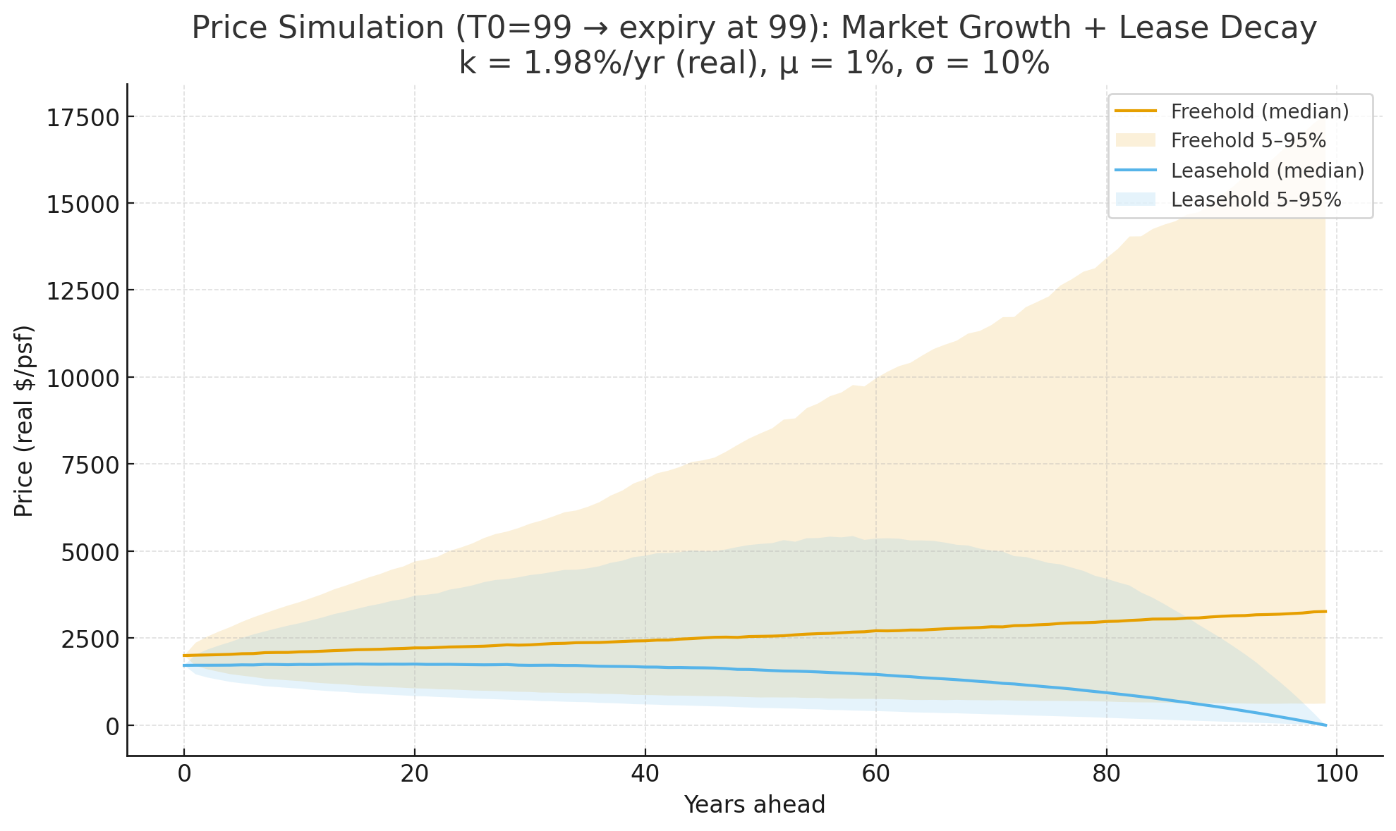
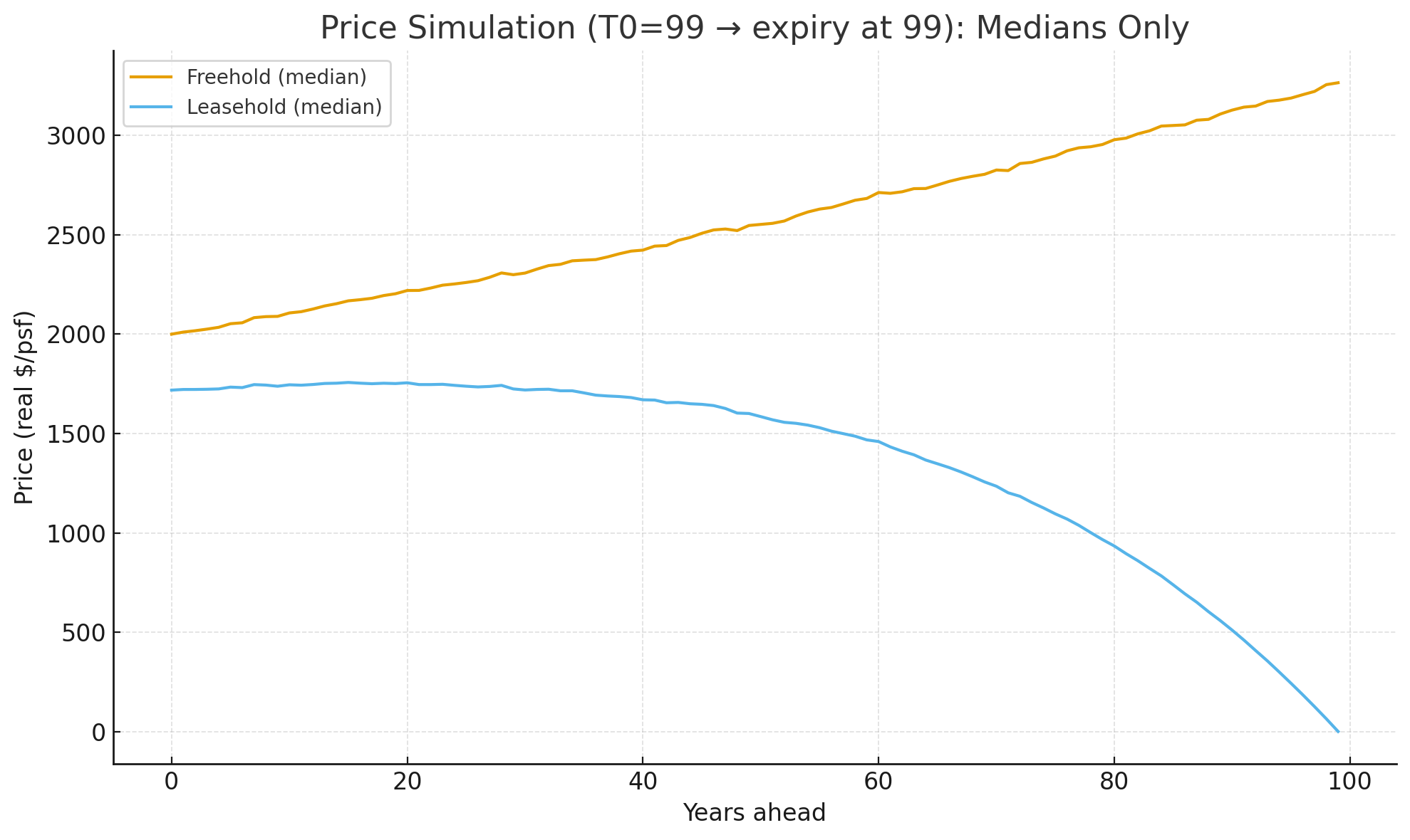
Median leasehold property values typically rise during the first 30 years before starting to decline. Their growth rate is also slower than that of freehold properties. Nonetheless, these trends can vary; for instance, the value tends to decline from around 60 years onwards at approximately the ~95% percentile.