I Let a Neural Network Do My Feature Engineering — Then Made It Explain Itself

An experiment in automated feature discovery for credit risk: a sequential model trained on raw payment history, interrogated with explainability tools, and translated into 52 plain tabular features that closed the entire gap to the neural model on holdout. Spread across two calendar days — with the human time measured in hours, not weeks.
The job that eats our weeks
If you build behavioral risk models, you know the drill. The signal lives in history tables — millions of payment events, monthly card balances, bureau records — and the only way to feed that to a scorecard or GBM is to collapse it into aggregates: mean days past due in the last 6 months, max utilization ever, count of late payments in 12.
The pain is combinatorial. Every variable × every window (3/6/12/24 months) × every statistic (mean, max, count, trend) × every condition you can dream up. Thousands of candidates. Weeks of analyst time. And when you ship, a quiet doubt remains: what did we not think of?
So I ran an experiment around a simple inversion: what if the model does the searching, and the analyst only does the reading?
The idea: the network is the search engine, not the product
The plan had three stages, each with a hard, falsifiable criterion:
Train a sequential neural network on near-raw history — no hand-crafted aggregates anywhere in its inputs — and require it to beat a meaningful bar: validation AUC > 0.78. The data: a private competition dataset modeled on the well-known Home Credit Kaggle data — an application table plus six history tables; 246K applications, 8.1% bad (default) rate, 13.6M payment events plus card, point-of-sale and credit bureau tables. (The raw data can’t be redistributed, but the public Kaggle Home Credit dataset has the same shape if you want to reproduce the method.)
Interrogate the frozen model with explainability tooling and write down, in plain language, what it learned.
Rebuild the findings as ordinary tabular features, hand them to a plain LightGBM, and measure how much of the network’s edge they keep — on a holdout set touched exactly once.
The crucial design decision: the neural network was never the deliverable. The deliverable was the feature list. The deployable model at the end is a boring, governance-friendly GBM over named columns — the network exists only to search a hypothesis space no analyst can cover by hand.
One constraint made the whole thing meaningful: the network’s inputs were raw event streams (due date, paid date, amounts, statuses…), with only “unit fixes” added — paid minus due = delay, paid over due = ratio. No windows, no decays, no counts-over-time. If we had fed it engineered aggregates, interrogating it would just have echoed our own assumptions back at us.
What actually happened (including the failures)
A disclosure that matters for everything that follows: I directed an AI coding agent (Claude Code) through the entire build — it wrote the pipeline, ran the experiments, and drafted the analyses; my own keyboard time across the two days went into design decisions at the start, a long stream of “explain this to me” challenges in the middle, and reading findings and approving feature names at the end. The honest log matters more than the highlight reel:
The first model failed the gate. It stalled at 0.767 validation AUC — barely above the applications-only baseline of 0.763 (validation). Before burning more GPU time, I had a set of independent AI reviewer agents audit the data pipeline, each instructed to try to refute the others’ bug reports so only solid findings survived. Three silent scaling bugs were confirmed. The worst: a clipping step had collapsed every applicant’s age to the same constant. Age — one of the strongest variables in retail credit — had been deleted from the model, and nothing crashed; the model trained merrily at a plausible-looking AUC. If you take one engineering lesson from this post: scaling bugs don’t announce themselves. Audit the transformed arrays — nunique(), clip-saturation — not just the raw data.
Then the neural fusion head hit a ceiling. With the bugs fixed and standard tricks applied (an auxiliary head forcing the behavioral embedding to be predictive on its own; randomly hiding the application features during training so the model can’t lean on them), the network’s own head still topped out around 0.769 (validation). Neural nets are simply mediocre at flat tabular data, where GBMs shine. The fix was architectural honesty: keep the network as the sequence reader, freeze its 128-number behavioral embedding, and let a LightGBM do the fusion — raw application columns and embedding columns side by side. That, plus a small ensemble of encoder variants, passed the gate at 0.7816 (validation).
The interrogation: making the black box talk
This is the part I’d never done before, and it’s where the experiment earns its keep. Three tools plus one final probe, deliberately different in mechanism, all run on the frozen model:
1. Attribution (Integrated Gradients) decomposes the behavioral score into per-event, per-channel contributions — a points table for a model that has no points table. It told us where the model looks: payment amounts and delays dominate, concentrated in the most recent ~10–15 installments; the monthly view is read as a current portfolio snapshot (the top channel was scheduled future installments — forward commitment burden, not delinquency); bureau signal concentrates in how recently accounts were opened. Best of all, plotting attribution against time produced a forgetting curve per data source — payments decay fast, applications and bureau records slowly. The model had learned different memory lengths for different data, something a uniform “last 12 months” window would have flattened.
2. Counterfactual perturbation is stress-testing aimed at the model: edit real histories surgically, re-score, measure. Injecting a fresh 3-payment late streak: +14.8 percentage points of predicted default probability in the top-risk decile. The same streak placed 18 months back: +0.9. That ratio is a feature specification — recency-discounted delinquency with a half-life around five to six payments, which became a literal column (Σ late × 0.89^k, k = payments back from today). Deleting the older half of someone’s history — mostly clean events — raised their risk: tenure itself is protective. And the null results mattered just as much: chronic mild underpayment, days-past-due (DPD) on monthly statements, utilization trend — all moved the model barely at all. Each null is strong evidence (not proof — the network can miss things too) that a feature family isn’t worth building for this portfolio, with a measured justification attached.
3. Embedding analysis treats the model’s internal customer summary (the encoders’ 128-number embeddings, concatenated) as a map of “behavior space”. Clustering it produced six archetypes whose real default rates ran 2.4% to 25.3% — and here’s the insight I keep retelling: median DPD was ~zero in every archetype. 92% of eventual defaulters had no statement delinquency at all in the prior year. The 10× risk separation came from soft gradients — how early people pay (10 days early vs 5), how deep their history runs, their refusal history. The model invented a segmentation no DPD-based rule could see.
The embedding gave us one final probe, the strangest of the lot: take the model’s main internal risk axis (the combination of embedding numbers that best tracks its score) and regress it on ~23 statistics we could name. They explained 39% of its variance (linear R²). The other 61% was the model knowing something we had no words for — so we pulled the customers at the extremes of that unexplained direction and read their raw files like underwriters. Two patterns emerged that none of our standard vocabulary captured: same-day bursts of refused applications (8–14 refusals, specific rejection codes) and heavy external debt sitting on a thin internal file. Both became features. Both are the kind of thing you find in year three of working a portfolio, not week one.
The verdict
Each finding became one or more named features — 52 in total, every one with a provenance note linking it to the finding that motivated it, implemented in plain pandas with no neural network anywhere at inference. Then the only test that matters, on the untouched holdout (holdout numbers run a little below the validation figures quoted above — expected, and exactly why the holdout exists):
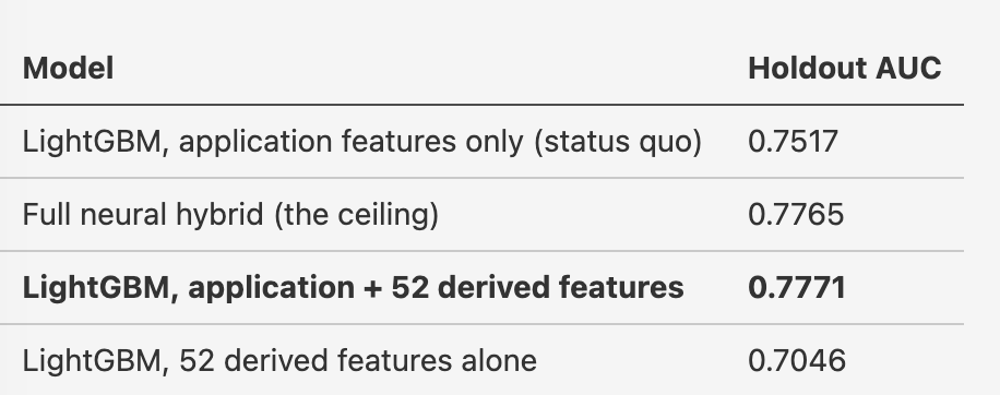
Gap closure: 102% on the point estimates — read that as a statistical tie: the 0.0006 AUC by which the features “beat” the network is well within noise on a single holdout, and I make nothing of it. The claim that matters is that the interpretable features kept essentially everything the network found (a second check agrees: the features-alone model matches the network’s behavior-only score head almost exactly). And no, that doesn’t make the network redundant: it found the features. Without it, the same list would have required exactly the manual search this experiment set out to replace.
Why I think this changes the feature-development workflow
Time. Two calendar days end-to-end, and most of that was compute, not human attention. The human’s job is compressed into: design decisions at the start, reading findings in the middle, naming features at the end.
Features arrive with evidence, not hunches. Every feature came with a measured functional form (the decay constant was fitted by the model and read off a dose-response curve, not guessed), a confirmed direction (useful for monotonicity constraints and model documentation), and — the underrated half — licensed omissions: measured evidence that the network, which saw everything, found no use for certain feature families, so nobody burns a sprint building them “just in case”.
Insights are a first-class output, not a by-product. The defaulters-look-clean finding, the archetype segmentation, the credit-appetite signal in bureau account openings — those are portfolio knowledge with uses far beyond one model: strategy, monitoring, collections prioritization. Manual feature engineering produces features; this produces features and an explanation of the portfolio.
The deployable artifact stays boring. Nothing about production changes: a GBM, named columns, documented provenance. For anyone working under model governance, that’s the difference between “interesting research” and “something I can actually ship”.
What this is not
Honesty section. The method is not human-free: someone chooses the raw representation, reads the extreme cases, and names the features — that’s the point, not a flaw (translation into human language requires a human). The perturbation effects are within-model sensitivities, not causal claims about customers. The probe is linear, so “61% unexplained” is an upper bound on mystery — some of it is interactions of known quantities. This is one dataset, one domain; the playbook needs adapting for very rare outcomes, drifting populations (use out-of-time holdouts!), or domains where the risk signal is what stopped happening. And it needs label volume — supervised embeddings want thousands of positives.
Also: I ran the interrogation as a single pass because that was the experiment’s design. In practice you’d loop — generate features, measure the remaining gap to the network, re-interrogate targeted at the cases where the features and the network disagree most, and repeat until converged. The disagreement cases are exactly where the unextracted signal hides.
Try it
The code and analysis are public: the full pipeline, the interrogation scripts, the findings documents with per-feature provenance, a tutorial written for risk professionals with no neural-network background, and a generalized, self-contained playbook for applying the method to other domains (churn, fraud, claims). The raw dataset itself can’t be redistributed — but the public Kaggle Home Credit data has the same shape if you want to run the method end to end:
https://github.com/kychanbp/auto-feature-gen-with-nn-interogation
My takeaway after two days: feature engineering didn’t disappear. It moved up a level — from writing thousands of candidate aggregates to reading what a model that saw everything chose to care about. I suspect that inversion is where the interesting work is moving.