Viewing Loan Core as a State Machine

How computational theory reveals the hidden order behind lending systems.

Oct 19, 2025

Loan management systems — or loan core — form the backbone of financial institutions. They govern the business logic behind loan creation, approval, disbursement, and repayment — in short, the entire loan cycle.

In abstract form, a loan core defines the states of a loan, the actions that can be taken (by users or by the system through auto-triggers), and the transitions between these states. When I began learning more about computational theory, it struck me that a loan core is, at its essence, a state machine.

It has to be — because a computer itself is a state machine. Viewing loan core from the lens of computational theory not only gives a formal framework for understanding how it works, but also helps navigate the various implementations across institutions. Beneath all the different designs and data structures, the logic can be abstracted into one thing: a finite state machine.

A Simplified Loan Core Example

Consider a minimal version of a loan core system.

A new loan starts in an initial state and moves through a sequence of states based on user actions or automated events:

[start] → (create) → [Pending] → (approve) → [Approved] → (disburse) → [Active] → (full repayment) → [Closed]
                            ↘ (reject)
                              [Rejected]

Each arrow represents a transition triggered by an event such as “approve” or “disburse.” The machine ensures that only valid transitions occur — for example, a loan can’t be disbursed before it’s approved.

A finite state machine (FSM) is, by definition, a machine that — at any given moment — is in a single state. When it receives an input, it looks up its transition table to determine the next state, and possibly what output or action to produce.

Formal Definition

Formally, a finite state machine can be defined as a five-tuple:

\(M = (Q, \Sigma, \delta, q_0, F)\)

where:

Q is the finite set of states.
Σ is the finite set of possible inputs (the alphabet).
δ is the transition function: ( Q × Σ → Q ).
q₀ ∈ Q is the start state.
F ⊆ Q is the set of accept (or terminal) states.

Applying this to our loan core system:

Q = { null, pending, approved, rejected, active, closed }
Σ = { create, approve, reject, disburse, full_repayment }
q₀ = null (start)
F = { rejected, closed }

Transition Table

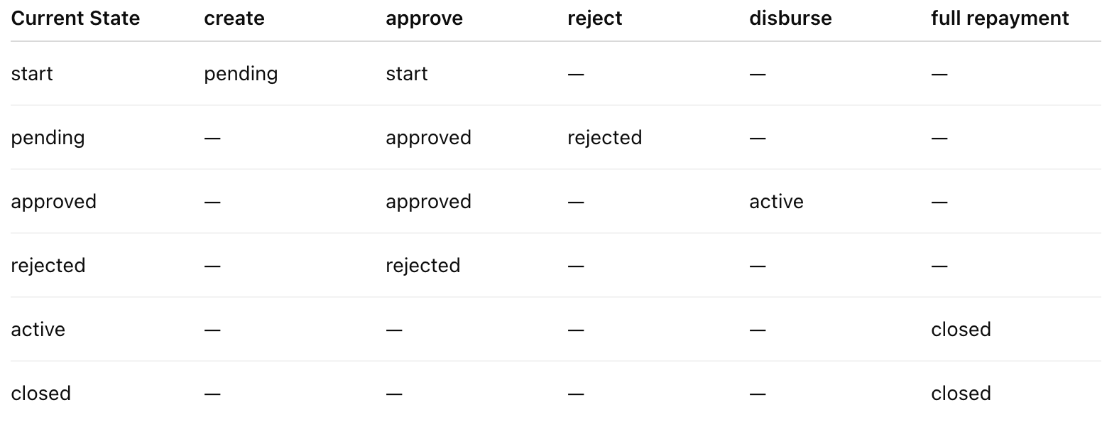
This simple table captures the essence of loan lifecycle logic — an ordered system of possible transitions bounded by rules. In practice, real-world loan cores are extended finite state machines (EFSMs), enriched with context variables, conditions, and side effects (for example, disbursing funds, updating ledgers, or sending notifications). But at their core, they remain recognizable as state machines — systems that transition deterministically between defined states.

From Theory to Reality: Apache Fineract

One open-source example that demonstrates this beautifully is Apache Fineract, a microfinance and loan management platform.
Fineract implements an extended state machine for loan lifecycle management. Each state (like Approved, Active, or Overpaid) can respond to a wide range of events — such as disbursal, repayment, write-off, or reschedule.

The following state transition matrix illustrates how complex this system becomes once we consider real-world business rules.

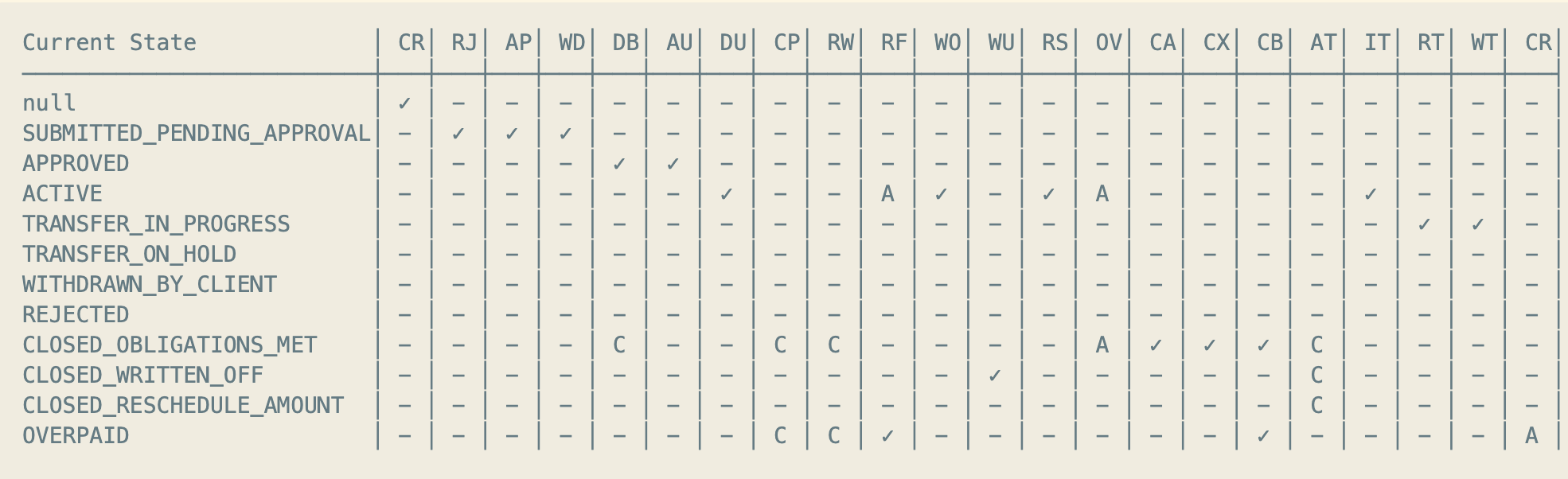
State Transition Matrix

Complete δ(Q, Σ) Matrix

This matrix shows all possible (state, event) combinations. Each cell contains the resulting state or an indicator of how the system handles that input. (This summary is genreated by Claude Code)

Legend:
✓ = Valid transition (always allowed)
C = Conditional transition (depends on context)
- = Invalid/blocked transition
A = Auto-transition (system-triggered)

Event Abbreviations:
CR=CREATED, RJ=REJECTED, AP=APPROVED, WD=WITHDRAWN, DB=DISBURSED
AU=APPROVAL_UNDO, DU=DISBURSAL_UNDO, CP=CHARGE_PAYMENT, RW=REPAYMENT_OR_WAIVER
RF=REPAID_IN_FULL, WO=WRITE_OFF, WU=WRITE_OFF_UNDO, RS=RESCHEDULE
OV=OVERPAYMENT, CA=CHARGE_ADDED, CX=CHARGE_ADJUSTMENT, CB=CHARGEBACK
AT=ADJUST_TRANSACTION, IT=INITIATE_TRANSFER, RT=REJECT_TRANSFER
WT=WITHDRAW_TRANSFER, CR=CREDIT_BALANCE_REFUND

Main Transition Matrix

From: SUBMITTED_AND_PENDING_APPROVAL (100)
├─ LOAN_REJECTED         → REJECTED (500)
├─ LOAN_APPROVED         → APPROVED (200)
└─ LOAN_WITHDRAWN        → WITHDRAWN_BY_CLIENT (400)

From: APPROVED (200)
├─ LOAN_DISBURSED        → ACTIVE (300)
└─ LOAN_APPROVAL_UNDO    → SUBMITTED_AND_PENDING_APPROVAL (100)

From: ACTIVE (300)
├─ LOAN_DISBURSAL_UNDO   → APPROVED (200)
├─ WRITE_OFF_OUTSTANDING → CLOSED_WRITTEN_OFF (601)
├─ LOAN_RESCHEDULE       → CLOSED_RESCHEDULE_OUTSTANDING_AMOUNT (602)
├─ LOAN_INITIATE_TRANSFER→ TRANSFER_IN_PROGRESS (303)
├─ REPAID_IN_FULL (auto) → CLOSED_OBLIGATIONS_MET (600) [if balance=0, charges paid]
└─ LOAN_OVERPAYMENT (auto)→ OVERPAID (700) [if totalOverpaid>0]

From: OVERPAID (700)
├─ LOAN_CREDIT_BALANCE_REFUND (auto) → CLOSED_OBLIGATIONS_MET (600) [if refunded]
├─ LOAN_CHARGE_PAYMENT   → ACTIVE (300) [if creates outstanding]
├─ LOAN_REPAYMENT_OR_WAIVER → ACTIVE (300) [if creates outstanding]
├─ LOAN_CHARGEBACK       → ACTIVE (300)
└─ REPAID_IN_FULL        → CLOSED_OBLIGATIONS_MET (600) [if conditions met]

From: CLOSED_OBLIGATIONS_MET (600)
├─ LOAN_DISBURSED        → ACTIVE (300) [multi-disburse only]
├─ LOAN_CHARGE_ADDED     → ACTIVE (300)
├─ LOAN_CHARGEBACK       → ACTIVE (300)
├─ LOAN_CHARGE_ADJUSTMENT→ OVERPAID (700) [if creates overpayment]
├─ LOAN_CHARGE_PAYMENT   → ACTIVE (300) [if creates outstanding]
├─ LOAN_REPAYMENT_OR_WAIVER → ACTIVE (300) [if creates outstanding]
├─ LOAN_ADJUST_TRANSACTION → ACTIVE (300) or OVERPAID (700) [depends on result]
└─ LOAN_OVERPAYMENT (auto)→ OVERPAID (700) [if totalOverpaid>0]

From: CLOSED_WRITTEN_OFF (601)
├─ WRITE_OFF_OUTSTANDING_UNDO → ACTIVE (300)
└─ LOAN_ADJUST_TRANSACTION → ACTIVE (300) or OVERPAID (700) [depends on result]

From: CLOSED_RESCHEDULE_OUTSTANDING_AMOUNT (602)
└─ LOAN_ADJUST_TRANSACTION → ACTIVE (300) or OVERPAID (700) [depends on result]

From: TRANSFER_IN_PROGRESS (303)
├─ LOAN_REJECT_TRANSFER  → TRANSFER_ON_HOLD (304)
└─ LOAN_WITHDRAW_TRANSFER→ ACTIVE (300)

From: REJECTED (500)
└─ [No transitions - terminal]

From: WITHDRAWN_BY_CLIENT (400)
└─ [No transitions - terminal]

From: TRANSFER_ON_HOLD (304)
└─ [No transitions - terminal]

Seeing Systems as State Machines

Modeling a system as a state machine is not just an academic exercise — it’s a way of thinking. It forces every assumption about what can happen, when, and under what conditions to become explicit. The loan core stops being a black box of code and business rules, and turns into a living map of states and transitions. You can reason about it, test it, simulate it, and explain it. Most importantly, it gives teams a shared grammar for complexity — engineers, risk analysts, and operations staff can finally point to the same table and agree on what “Active” or “Closed” really means.

Beyond the State Machine

The state machine captures the skeleton of the loan core — the structure of states and valid transitions. But the living body of the system includes many other organs working in sync.

At the heart of it are transaction functions that handle money movement: disbursement, repayment, fees, and penalties. Each of these operations changes not only account balances but also the loan’s internal context — triggering new transitions in the state machine.

Surrounding this are repayment schedule generators, which determine expected installments and interest accruals; and fee and penalty managers. Beyond the core logic, other crucial layers complete the ecosystem:

Account management, which maintains borrower and product relationships.
Accounting, which records journal entries and enforces financial integrity.
API and service layers, which expose the system’s functions to external modules like mobile apps or credit platforms.

Thinking in FSM terms doesn’t replace these subsystems — it organizes them. The state machine becomes the control plane that orchestrates when and how these modules act. By defining the legal transitions clearly, every financial operation — from posting a repayment to writing off a loan — has a well-defined place in the broader choreography.

ZhiZhi Gewu

Discussion about this post