What's Really Going On in Machine Learning? A Simplest Example by Stephen Wolfram
From Neural Networks to Rule Arrays: A Minimal Model of Learning

In a Neural Net (NN)[1], the standard setup includes an input layer, hidden layers that sit between the input and output layer, and neurons that contain the weights, a bias, and a reference to the activation function. The architecture defines the computation graph (visually, that is, the connections between nodes); the forward pass evaluates that graph for a given input. Back-propagation computes gradients of the loss with respect to the parameters; an optimizer such as SGD or Adam then updates the weights.
To understand it, we can simplify as many components as possible. First, let’s restrict connections to local neighbors only — for example, the Mesh Neural Net. Second, let’s make everything discrete instead of continuous. The simplest discrete analog is a rule array — a cellular-automaton-like grid in which each cell independently picks which rule to apply from a small fixed panel (see Appendix for an introduction to cellular automata). The value of a cell is discrete: either 1 or 0. The value of the cell depends on the left, center, and right cells preceding it by a rule set. Analogously, each cell in the grid is a neuron in NN. The row in the grid is the layers. The computation graph is constructed as a mesh network that depends on local neighbors. Random mutation is analogous to a training/optimization procedure, but unlike gradient descent, it does not use gradients. It is closer to stochastic hill climbing or evolutionary search. The value of the cell is similar to activation, the value the neuron produces after the forward pass computation.
Implementation
First, we defined the grid size to be \((T, W) = (60, 60)\) where \(T\) is the number of time steps and \(W\) is the width of the grid.
Second, we define a function to generate the rule set, converting decimal to binary (see Appendix for details).
def rule_to_lut(n):
    """Convert rule number to a lookup table."""
    return [ (n // 2**i) % 2 for i in range(8) ]
We will mainly use rule 4 and rule 146. The lookup tables are:
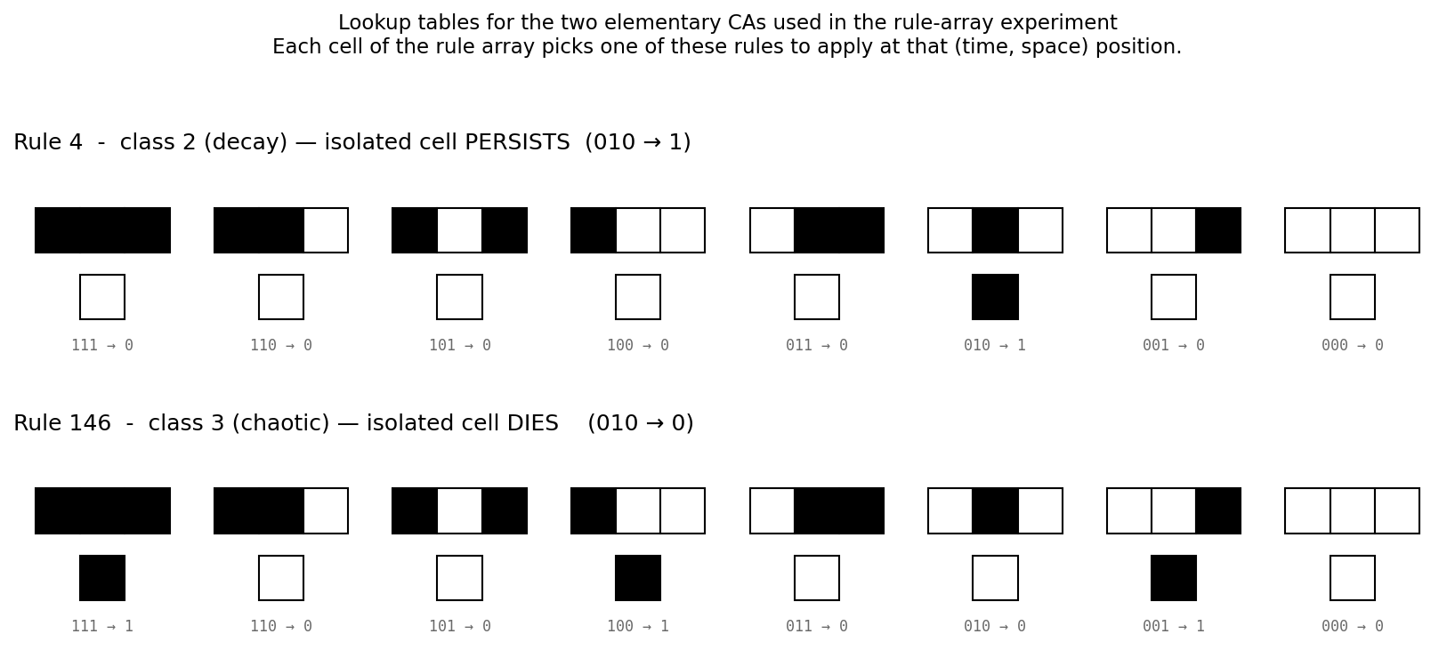
Third, we construct a rule array that indicates whether to apply rule 4 or rule 146 to each cell, and initialize it to zeros.
rule_array = [[0] * W for _ in range(T)]Fourth, we define a function to evolve the row one by one in the grid, starting with the initial configuration [0000...010...0000]. Then, we loop through the cell from top to bottom and left to right, and apply the corresponding rule set (Rule 4 or Rule 146) based on the value in the rule array (0 or 1).
def evolve(rule_array, initial_row):
    T = len(rule_array)
    W = len(initial_row)
    pat = [list(initial_row)]  # start with the initial row
    for t in range(T):  # loop through time steps
        new_row = []
        for w in range(W):  # loop through cell width
            left = pat[t][w-1] if w-1 >= 0 else pat[t][W-1]  # if hitting left wall, treat as the rightmost cell
            center = pat[t][w]
            right = pat[t][w+1] if w+1 < W else pat[t][0]  # if hitting right wall, treat as the leftmost cell
            idx = left * 4 + center * 2 + right  # convert binary to decimal index

            if rule_array[t][w] == 0:
                new_row.extend([rule_4_lut[idx]])  # apply rule 4
            else:
                new_row.extend([rule_146_lut[idx]])  # apply rule 146
        pat.append(new_row)

    return pat
Fifth, we have to define our loss function. Our goal is to have a Cellular Automata that stops at a certain lifetime, say 30. The definition of lifetime is the index of the last nonzero row. The loss is just the absolute difference between our target and our lifetime.
def lifetime(pat):
    """Calculate the lifetime of the pattern."""

    for t in range(len(pat) - 1, -1, -1):  # start from the last time step; -1 means go backwards; -1 means stop at the first time step
        if any(pat[t]):
            return t
    return 0

def loss(rule_array, target):
    pat = evolve(rule_array, initial_row)
    return abs(lifetime(pat) - target)
Finally, we have to write our training loop that mutates the rule array, similar to how we find the weights in the NN. We start by initializing the rule_array randomly, then flip the bit in the array if the loss is less than or equal to the current loss. The reason to use <= instead of < is that by including the run with the same loss, we avoid getting stuck in the same mutation (weights).
def train(target, max_steps=10000):

    random_rule_array = [[random.choice([0, 1]) for _ in range(W)] for _ in range(T)]  # Initialize a random rule array
    current_loss = loss(random_rule_array, target)
    loss_history = [current_loss]

    for step in range(max_steps):
        # Randomly flip a bit in the rule array
        t = random.randint(0, T-1)
        w = random.randint(0, W-1)
        random_rule_array[t][w] = 1 - random_rule_array[t][w]  # 1-0 = 1 and 1-1 = 0, so this effectively flips the bit

        new_loss = loss(random_rule_array, target)

        if new_loss == 0:
            current_loss = new_loss
            loss_history.append(current_loss)
            break
        elif new_loss <= current_loss:
            current_loss = new_loss
            loss_history.append(current_loss)
        else:  # Revert the change if it doesn't improve the loss
            random_rule_array[t][w] = 1 - random_rule_array[t][w]
            loss_history.append(current_loss)

    return random_rule_array, loss_history
Results and Implications
We can observe that the simplified NN construction did “learn.” However, the solutions seem to have no pattern. Somehow, some rules did minimize the loss function. In fact, the simplest solution is to apply only one rule-146 in row 30.
The main messages from the book by Stephen are:
Many trained systems do not work by discovering clean, human-readable mechanisms. Training is an adaptive process that searches an enormous computational space and retains any behavior that happens to align with the constraints.
ML works because of computational irreducibility (the concept introduced by Stephen Wolfram in A New Kind of Science). You cannot shortcut their behavior with a closed-form theory. ML exploits this by exploring the vast, irreducible computational space, which almost always finds one whose dynamics satisfy the need.
There is a trade-off between explainability (for example, a closed-form solution) and performance, because if we require explainability, we restrict the search in computational irreducible space.
Appendix: Cellular Automata
A one-dimensional Cellular Automata (CA) of two states starts with an array of ones and zeros. The next generation (the next row) is generated by a set of rules that take two adjacent cells and itself as inputs, and output the next cell.
Since there are \(2^3 = 8\) combinations of inputs, the rule set can be expressed in 8 digits. For example, binary 00011110 = decimal 30; this is called Rule 30 (see Appendix: Base Conversion for more information). Therefore, there are, in total, \(2^8 = 256\) possible rule sets.
For example, the following is the space-time pattern[2] of Rule 30:
Appendix: Base Conversion
In Python, the conversion can be achieved in one line by answering whether \(2^i\) is in the sum. \(2^7\) is in the sum, while \(2^6\) is not, as we saw above. It is easier to see in base-10 first. To answer whether \(40\) is in the sum of \(146\) (\(146 = 100 + 40 + 6\)) — in other words, what is the tens digit of \(146\) — we can first chop off the last digit (mathematically, \(146 \,//\, 10\)[4]) and look at the rightmost digit of what’s left (mathematically, \(146 \,//\, 10 \bmod 10 = 4\)[5]). Applying the same logic to base-2 of number \(n\), it becomes \(n \,//\, 2^i \bmod 2\).
Appendix: Code
Polish by Claude:
"""
Wolfram §5 replication — train a rule array to a target lifetime.
Replicates the lifetime-training experiment from Stephen Wolfram,
*What's Really Going On in Machine Learning? Some Minimal Models* (2025),
Section 5 ("Machine Learning in Discrete Rule Arrays").
Each cell of a T x W rule array selects between two elementary cellular
automata (rule 4, decay; rule 146, chaotic) to apply at that (time, space)
position. From a single black cell in row 0, the pattern evolves forward T
steps. Training searches for a rule array whose pattern survives EXACTLY
`target` steps, using single-point mutation hill-climbing with the rule
"accept iff new loss <= old loss". The equality is what lets the search
drift across plateaus until it stumbles into a downhill move.
Phenomena reproduced:
1. Random mutation actually trains.
2. Trained rule arrays look like noise (no obvious mechanism).
3. Different runs find different solutions.
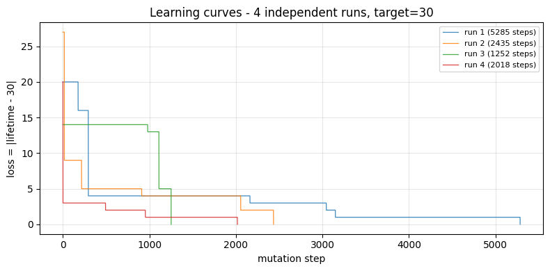
4. Plateau-and-breakthrough learning curves.
5. Engineered solutions exist but training does not discover them.
Outputs (under --out-dir, default = script directory):
- learning_curves.png loss vs. mutation step, all runs overlaid
- trained_runs.png trained rule arrays + spacetime patterns
- trained_spacetime.gif animated row-by-row evolution
Usage:
python wolfram_lifetime.py
python wolfram_lifetime.py --t 30 --w 30 --target 15 --max-steps 10000
python wolfram_lifetime.py --no-gif
"""
from __future__ import annotations
import argparse
import random
from pathlib import Path
import numpy as np
import matplotlib.pyplot as plt
from matplotlib.animation import FuncAnimation, PillowWriter
# -----------------------------------------------------------------------------
# Elementary cellular automata
# -----------------------------------------------------------------------------
def rule_to_lut(n: int) -> list[int]:
"""8-entry lookup table for an elementary (k=2, r=1) CA.
Indexed by (left << 2) | (center << 1) | right."""
return [(n >> i) & 1 for i in range(8)]
RULE_4_LUT = rule_to_lut(4) # class 2 -- decay
RULE_146_LUT = rule_to_lut(146) # class 3 -- chaotic
def evolve(rule_array: list[list[int]], initial_row: list[int]) -> list[list[int]]:
"""Run the 1D CA forward, selecting rule 4 or rule 146 per cell.
`rule_array[t][w]` selects which rule applies at time t, column w
(0 -> rule 4, 1 -> rule 146). Width is cyclic.
Returns the spacetime pattern: a (T+1) x W list of lists.
"""
T = len(rule_array)
W = len(initial_row)
pat = [list(initial_row)]
for t in range(T):
prev = pat[t]
new_row = [0] * W
for w in range(W):
# cyclic neighborhood: modulo handles both walls
idx = (prev[(w - 1) % W] << 2) | (prev[w] << 1) | prev[(w + 1) % W]
lut = RULE_4_LUT if rule_array[t][w] == 0 else RULE_146_LUT
new_row[w] = lut[idx]
pat.append(new_row)
return pat
def lifetime(pat: list[list[int]]) -> int:
"""Largest row index containing any black cell. 0 if dead from the start."""
for t in range(len(pat) - 1, -1, -1):
if any(pat[t]):
return t
return 0
# -----------------------------------------------------------------------------
# Training: single-point mutation hill climbing
# -----------------------------------------------------------------------------
def loss(rule_array: list[list[int]], initial_row: list[int], target: int) -> int:
return abs(lifetime(evolve(rule_array, initial_row)) - target)
def train(
target: int,
T: int,
W: int,
initial_row: list[int],
max_steps: int = 20_000,
seed: int | None = None,
) -> tuple[list[list[int]], list[int]]:
"""Hill-climb a rule array to lifetime = target.
Starts from a random binary rule array of shape (T, W). Each iteration
flips one random cell; the flip is kept iff `new_loss <= cur_loss` (the
`<=` is what lets the search cross plateaus). Early-stops on loss == 0.
Returns (trained_rule_array, loss_history). The history has one entry
per iteration, so its length equals the number of mutations attempted
(+ 1 for the initial state).
"""
rng = random.Random(seed)
arr = [[rng.randint(0, 1) for _ in range(W)] for _ in range(T)]
cur_loss = loss(arr, initial_row, target)
history = [cur_loss]
for _ in range(max_steps):
i, j = rng.randrange(T), rng.randrange(W)
arr[i][j] = 1 - arr[i][j] # flip
new_loss = loss(arr, initial_row, target)
if new_loss <= cur_loss:
cur_loss = new_loss
else:
arr[i][j] = 1 - arr[i][j] # revert
history.append(cur_loss)
if cur_loss == 0:
break
return arr, history
# -----------------------------------------------------------------------------
# Visualization
# -----------------------------------------------------------------------------
def plot_learning_curves(runs, target: int, out_path: Path) -> None:
"""Loss vs. mutation step for all runs, overlaid."""
fig, ax = plt.subplots(figsize=(8, 4))
for k, (_, hist) in enumerate(runs):
ax.plot(hist, lw=0.9, alpha=0.85, label=f"run {k+1} ({len(hist)-1} steps)")
ax.set_xlabel("mutation step")
ax.set_ylabel(f"loss = |lifetime - {target}|")
ax.set_title(f"Learning curves - {len(runs)} independent runs, target={target}")
ax.legend(fontsize=8)
ax.grid(alpha=0.3)
fig.tight_layout()
fig.savefig(out_path, dpi=150, bbox_inches="tight")
plt.close(fig)
def plot_trained_runs(runs, initial_row, target: int, out_path: Path) -> None:
"""Trained rule arrays (top) and their spacetime patterns (bottom)."""
n = len(runs)
fig, axes = plt.subplots(2, n, figsize=(3 * n, 7.2), constrained_layout=True)
if n == 1:
axes = axes.reshape(2, 1)
for k, (arr, hist) in enumerate(runs):
axes[0, k].imshow(arr, cmap="binary", aspect="equal",
interpolation="nearest", vmin=0, vmax=1)
axes[0, k].set_title(f"run {k+1}: rule array\n({len(hist)-1} mutations)",
fontsize=10)
axes[0, k].set_xticks([]); axes[0, k].set_yticks([])
if k == 0:
axes[0, k].set_ylabel("LEARNED\nrule array\n(black=146, white=4)",
fontsize=9)
pat = evolve(arr, initial_row)
axes[1, k].imshow(pat, cmap="binary", aspect="equal",
interpolation="nearest", vmin=0, vmax=1)
axes[1, k].axhline(target + 0.5, color="red", lw=1.0, ls="--",
alpha=0.8, label=f"target row {target}")
axes[1, k].set_title(f"spacetime (lifetime {lifetime(pat)})", fontsize=10)
axes[1, k].set_xticks([]); axes[1, k].set_yticks([])
if k == 0:
axes[1, k].set_ylabel("RESULTING\nspacetime\n(time flows down)",
fontsize=9)
axes[1, k].legend(loc="lower right", fontsize=7)
fig.suptitle(
f"Wolfram §5 replication - {n} independent training runs, target lifetime = {target}\n"
"Each run learns a different rule array; spacetimes are unrelated but all die at the target row.",
fontsize=11,
)
fig.savefig(out_path, dpi=150, bbox_inches="tight")
plt.close(fig)
def animate_trained_runs(
runs, initial_row, target: int, out_path: Path, fps: int = 5
) -> None:
"""Animated gif: rule array (top) and spacetime (bottom) reveal in lockstep,
one row per frame. Rule-array row t produces spacetime row t+1.
"""
n = len(runs)
arrs = [np.array(arr) for arr, _ in runs]
pats = [np.array(evolve(arr, initial_row)) for arr, _ in runs]
lifetimes = [lifetime(p.tolist()) for p in pats]
mutations = [len(h) - 1 for _, h in runs]
n_frames = pats[0].shape[0] # T + 1
fig, axes = plt.subplots(2, n, figsize=(3 * n, 6.6))
if n == 1:
axes = axes.reshape(2, 1)
fig.subplots_adjust(top=0.86, bottom=0.04, left=0.06, right=0.98,
hspace=0.25, wspace=0.10)
def render(t):
for k in range(n):
ax_top = axes[0, k]
ax_top.clear()
ax_top.set_xticks([]); ax_top.set_yticks([])
ax_top.set_title(
f"run {k+1}: rule array\n({mutations[k]} mutations)", fontsize=10
)
display_arr = np.zeros_like(arrs[k])
if t > 0:
display_arr[:t] = arrs[k][:t]
ax_top.imshow(display_arr, cmap="binary", aspect="equal",
interpolation="nearest", vmin=0, vmax=1)
if k == 0:
ax_top.set_ylabel("LEARNED\nrule array\n(black=146, white=4)",
fontsize=9)
ax_bot = axes[1, k]
ax_bot.clear()
ax_bot.set_xticks([]); ax_bot.set_yticks([])
ax_bot.set_title(f"spacetime (lifetime {lifetimes[k]})", fontsize=10)
display_pat = np.zeros_like(pats[k])
display_pat[: t + 1] = pats[k][: t + 1]
ax_bot.imshow(display_pat, cmap="binary", aspect="equal",
interpolation="nearest", vmin=0, vmax=1)
ax_bot.axhline(target + 0.5, color="red", lw=1.0, ls="--",
alpha=0.8, label=f"target row {target}")
if k == 0:
ax_bot.set_ylabel("RESULTING\nspacetime\n(time flows down)",
fontsize=9)
ax_bot.legend(loc="lower right", fontsize=7)
fig.suptitle(
f"Wolfram §5 replication - {n} independent training runs, "
f"target lifetime = {target} - step {t}/{n_frames - 1}\n"
"Each run learns a different rule array; spacetimes are unrelated "
"but all die at the target row.",
fontsize=11,
y=0.985,
)
anim = FuncAnimation(fig, render, frames=n_frames, interval=1000 // fps)
anim.save(out_path, writer=PillowWriter(fps=fps))
plt.close(fig)
# -----------------------------------------------------------------------------
# Main
# -----------------------------------------------------------------------------
def main() -> None:
ap = argparse.ArgumentParser(
description="Train a rule array to a target lifetime (Wolfram §5)."
)
ap.add_argument("--t", type=int, default=60, help="time steps (rule-array rows)")
ap.add_argument("--w", type=int, default=60, help="width (rule-array cols)")
ap.add_argument("--target", type=int, default=30, help="target lifetime")
ap.add_argument("--max-steps", type=int, default=20_000,
help="max mutations per run")
ap.add_argument("--n-runs", type=int, default=4,
help="number of independent training runs")
ap.add_argument("--seed", type=int, default=7,
help="base seed (per-run seeds are derived)")
ap.add_argument("--out-dir", type=Path,
default=Path(__file__).resolve().parent,
help="where to save figures")
ap.add_argument("--no-gif", action="store_true",
help="skip the animated gif (faster)")
args = ap.parse_args()
if not 0 <= args.target <= args.t:
raise SystemExit(f"target must be in [0, {args.t}]; got {args.target}")
initial_row = [0] * args.w
initial_row[args.w // 2] = 1
rng = random.Random(args.seed)
seeds = [rng.randrange(10**9) for _ in range(args.n_runs)]
print(f"Training {args.n_runs} runs at T={args.t}, W={args.w}, target={args.target}...")
runs = []
for k, s in enumerate(seeds):
arr, hist = train(
args.target, args.t, args.w, initial_row,
max_steps=args.max_steps, seed=s,
)
lt = lifetime(evolve(arr, initial_row))
print(f" run {k+1} seed={s}: final loss={hist[-1]}, "
f"lifetime={lt}, mutations={len(hist) - 1}")
runs.append((arr, hist))
args.out_dir.mkdir(parents=True, exist_ok=True)
plot_learning_curves(runs, args.target, args.out_dir / "learning_curves.png")
plot_trained_runs(runs, initial_row, args.target,
args.out_dir / "trained_runs.png")
print(f"Saved learning_curves.png and trained_runs.png to {args.out_dir}")
if not args.no_gif:
animate_trained_runs(runs, initial_row, args.target,
args.out_dir / "trained_spacetime.gif")
print(f"Saved trained_spacetime.gif to {args.out_dir}")
if __name__ == "__main__":
main()
Footnotes
[1] If readers are not familiar with NN, here is a great introduction: 3Blue1Brown — But what is a neural network?.
[2] The column is space, and the row is time.
[3] In the case of a list in Python, we usually write from left to right.
[4] Integer division.
[5] Modulo.